November 23, 2025

Simulating Time: How to Hand-Craft Chrome Trace Viewer JSON for Visualization

It’s been a few months since I came to Toronto. The weather has cooled off a bit lately. Earlier this November, we experienced the earliest first snowfall here in the past 56 years. It’s warmed up slightly since then, with an average temperature around 3°C to 6°C, pretty comfortable, just right for a hoodie and a light coat. By the way, I might need to buy another pair of snow boots.
Hong-Sheng Zheng, November 23, 2025

This post introduces a useful visualization tool for timeline tracing: Chrome Trace Viewer. You can open the tool with the URL chrome://tracing, and you can use it directly in your chrome-based browser. If you are new to this tool, after loading a JSON file into the viewer, try pressing “W”, “A”, “S”, “D” to navigate around, these are the common keyboard shortcuts for panning and zooming the timeline.

This project was developed by the Google Chrome team and has now evolved into the more advanced Perfetto. Both tools can ingest data in the same JSON format, so don’t worry about which one you use. These tools allow you to observe the execution timeline of your program. When I was an AI compiler engineer at MediaTek, I frequently used these charts to help me analyze performance across different engines, so I can explore parallelism, workload balance, and so on, to determine how to further optimize programs. 😀

An Example

Before diving deep into the format for the trace viewer, let me start with an example.
Imagine a data processing flow: Load → Compute → Store. Each stage is handled by a different engine, and data transmission is streaming:

Load: Uses ping-pong buffering, allowing the system to pre-load an extra buffer ahead of time.
Compute: Does not need to wait for the Load phase to fully complete; it can start processing early (overlapped execution).
Store: Similarly, it can transfer small chunks of processed data to the Store engine for write-back immediately.

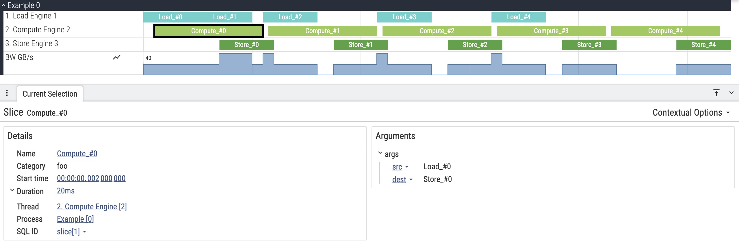
In this chart, we also show the memory bandwidth, which indicates whether the current program has hit the memory bandwidth limit. Here, we show a compute-bound example, that the computation time dominates the whole program execution.

Compared to raw statistical results, a visual chart is significantly more readable. Hmm… Has anyone else heard of the “Coke vs. Tea” theory? I can’t quite remember where I first encountered this idea 🥸, but it just illustrates the law of Diminishing Marginal Utility. The theory goes that the first sip of Coke provides the maximum rush of satisfaction, but that feeling drops precipitously with every subsequent sip. So the satisfaction you get from drinking a large bottle of Coke is roughly the same as drinking a small can of Coke; the extra volume does not increase happiness. Similarly, these charts were exciting to look at initially, but they can become exhausting when you’re deeply involved in identifying optimization issues every day 😅

Understanding the Trace Event Format

To generate this chart, you need to understand the JSON format used by Trace Viewer. Here is the structure of the data shown in the image above. You can copy it and try it. The most important component is the traceEvents array. You can read the full specification here: Trace Event Format

{
    "displayTimeUnit": "ns",
    "traceEvents": [
        { "name": "process_name", "ph": "M", "pid": 0, "tid": 0, "args": { "name": "Example" } },

        { "name": "thread_name", "ph": "M", "pid": 0, "tid": 1,
          "args": { "name": "1. Load Engine" } },
        { "name": "thread_name", "ph": "M", "pid": 0, "tid": 2,
          "args": { "name": "2. Compute Engine" } },
        { "name": "thread_name", "ph": "M", "pid": 0, "tid": 3,
          "args": { "name": "3. Store Engine" } },
        { "name": "thread_name", "ph": "M", "pid": 0, "tid": 4,
          "args": { "name": "4. Memory Bandwidth" } },

        { "name": "Load_#0", "cat": "foo", "ph": "B", "ts": 0, "pid": 0, "tid": 1,
          "args": { "dest": "Compute_#0" }},
        { "name": "Load_#0", "cat": "foo", "ph": "E", "ts": 10000, "pid": 0, "tid": 1},
        { "name": "Compute_#0", "cat": "foo", "ph": "B", "ts": 2000, "pid": 0, "tid": 2,
          "args": { "src": "Load_#0", "dest": "Store_#0" }},
        { "name": "Compute_#0", "cat": "foo", "ph": "E", "ts": 22000, "pid": 0, "tid": 2},
        { "name": "Store_#0", "cat": "foo", "ph": "B", "ts": 14000, "pid": 0, "tid": 3,
          "args": { "src": "Compute_#0" }},
        { "name": "Store_#0", "cat": "foo", "ph": "E", "ts": 24000, "pid": 0, "tid": 3},

        { "name": "Load_#1", "cat": "foo", "ph": "B", "ts": 10000, "pid": 0, "tid": 1,
          "args": { "dest": "Compute_#1" }},
        { "name": "Load_#1", "cat": "foo", "ph": "E", "ts": 20000, "pid": 0, "tid": 1 },
        { "name": "Compute_#1", "cat": "foo", "ph": "B", "ts": 23000, "pid": 0, "tid": 2,
          "args": { "src": "Load_#1", "dest": "Store_#1" } },
        { "name": "Compute_#1", "cat": "foo", "ph": "E", "ts": 43000, "pid": 0, "tid": 2 },
        { "name": "Store_#1", "cat": "foo", "ph": "B", "ts": 35000, "pid": 0, "tid": 3,
          "args": { "src": "Compute_#1" } },
        { "name": "Store_#1", "cat": "foo", "ph": "E", "ts": 45000, "pid": 0, "tid": 3 },

        { "name": "Load_#2", "cat": "foo", "ph": "B", "ts": 22000, "pid": 0, "tid": 1,
          "args": { "dest": "Compute_#2" } },
        { "name": "Load_#2", "cat": "foo", "ph": "E", "ts": 32000, "pid": 0, "tid": 1 },
        { "name": "Compute_#2", "cat": "foo", "ph": "B", "ts": 44000, "pid": 0, "tid": 2,
          "args": { "src": "Load_#2", "dest": "Store_#2" } },
        { "name": "Compute_#2", "cat": "foo", "ph": "E", "ts": 64000, "pid": 0, "tid": 2 },
        { "name": "Store_#2", "cat": "foo", "ph": "B", "ts": 56000, "pid": 0, "tid": 3,
          "args": { "src": "Compute_#2" } },
        { "name": "Store_#2", "cat": "foo", "ph": "E", "ts": 66000, "pid": 0, "tid": 3 },

        { "name": "Load_#3", "cat": "foo", "ph": "B", "ts": 43000, "pid": 0, "tid": 1,
          "args": { "dest": "Compute_#3" } },
        { "name": "Load_#3", "cat": "foo", "ph": "E", "ts": 53000, "pid": 0, "tid": 1 },
        { "name": "Compute_#3", "cat": "foo", "ph": "B", "ts": 65000, "pid": 0, "tid": 2,
          "args": { "src": "Load_#3", "dest": "Store_#3" } },
        { "name": "Compute_#3", "cat": "foo", "ph": "E", "ts": 85000, "pid": 0, "tid": 2 },
        { "name": "Store_#3", "cat": "foo", "ph": "B", "ts": 77000, "pid": 0, "tid": 3,
          "args": { "src": "Compute_#3" } },
        { "name": "Store_#3", "cat": "foo", "ph": "E", "ts": 87000, "pid": 0, "tid": 3 },

        { "name": "Load_#4", "cat": "foo", "ph": "B", "ts": 64000, "pid": 0, "tid": 1,
          "args": { "dest": "Compute_#4" } },
        { "name": "Load_#4", "cat": "foo", "ph": "E", "ts": 74000, "pid": 0, "tid": 1 },
        { "name": "Compute_#4", "cat": "foo", "ph": "B", "ts": 86000, "pid": 0, "tid": 2,
          "args": { "src": "Load_#4", "dest": "Store_#4" } },
        { "name": "Compute_#4", "cat": "foo", "ph": "E", "ts": 106000, "pid": 0, "tid": 2 },
        { "name": "Store_#4", "cat": "foo", "ph": "B", "ts": 98000, "pid": 0, "tid": 3,
          "args": { "src": "Compute_#4" } },
        { "name": "Store_#4", "cat": "foo", "ph": "E", "ts": 108000, "pid": 0, "tid": 3 },

        { "name": "BW", "ph": "C", "ts": 0, "pid": 0, "tid": 4, "args": { "GB/s": 20 } },
        { "name": "BW", "ph": "C", "ts": 14000, "pid": 0, "tid": 4, "args": { "GB/s": 40 } },
        { "name": "BW", "ph": "C", "ts": 20000, "pid": 0, "tid": 4, "args": { "GB/s": 20 } },
        { "name": "BW", "ph": "C", "ts": 22000, "pid": 0, "tid": 4, "args": { "GB/s": 40 } },
        { "name": "BW", "ph": "C", "ts": 24000, "pid": 0, "tid": 4, "args": { "GB/s": 20 } },
        { "name": "BW", "ph": "C", "ts": 32000, "pid": 0, "tid": 4, "args": { "GB/s": 0 } },

        { "name": "BW", "ph": "C", "ts": 35000, "pid": 0, "tid": 4, "args": { "GB/s": 20 } },
        { "name": "BW", "ph": "C", "ts": 43000, "pid": 0, "tid": 4, "args": { "GB/s": 40 } },
        { "name": "BW", "ph": "C", "ts": 45000, "pid": 0, "tid": 4, "args": { "GB/s": 20 } },
        { "name": "BW", "ph": "C", "ts": 53000, "pid": 0, "tid": 4, "args": { "GB/s": 0 } },

        { "name": "BW", "ph": "C", "ts": 56000, "pid": 0, "tid": 4, "args": { "GB/s": 20 } },
        { "name": "BW", "ph": "C", "ts": 64000, "pid": 0, "tid": 4, "args": { "GB/s": 40 } },
        { "name": "BW", "ph": "C", "ts": 66000, "pid": 0, "tid": 4, "args": { "GB/s": 20 } },
        { "name": "BW", "ph": "C", "ts": 74000, "pid": 0, "tid": 4, "args": { "GB/s": 0 } },

        { "name": "BW", "ph": "C", "ts": 77000, "pid": 0, "tid": 4, "args": { "GB/s": 20 } },
        { "name": "BW", "ph": "C", "ts": 87000, "pid": 0, "tid": 4, "args": { "GB/s": 0 } },

        { "name": "BW", "ph": "C", "ts": 98000, "pid": 0, "tid": 4, "args": { "GB/s": 20 } },
        { "name": "BW", "ph": "C", "ts": 108000, "pid": 0, "tid": 4, "args": { "GB/s": 20 } }
    ]
}

Trace Event Parameters

Each trace event has the following parameters:

name: The name of the event
cat: Category. While not visually distinct, this is useful for filtering events with search.
ph: Phase, which determines how to interpret this event (There are five common events)
- “X”: Complete event with duration
- “M”: Metadata event
- “C”: Counter event
- “B”: Marks the beginning of an event.
- “E”: Marks the end of an event.
dur: Duration, the time spent on this event (used with phase “X”)
ts: Timestamp in microseconds (µs).
pid: Process ID
tid: Thread ID
args: Additional arguments/metadata for the event

Structure Overview

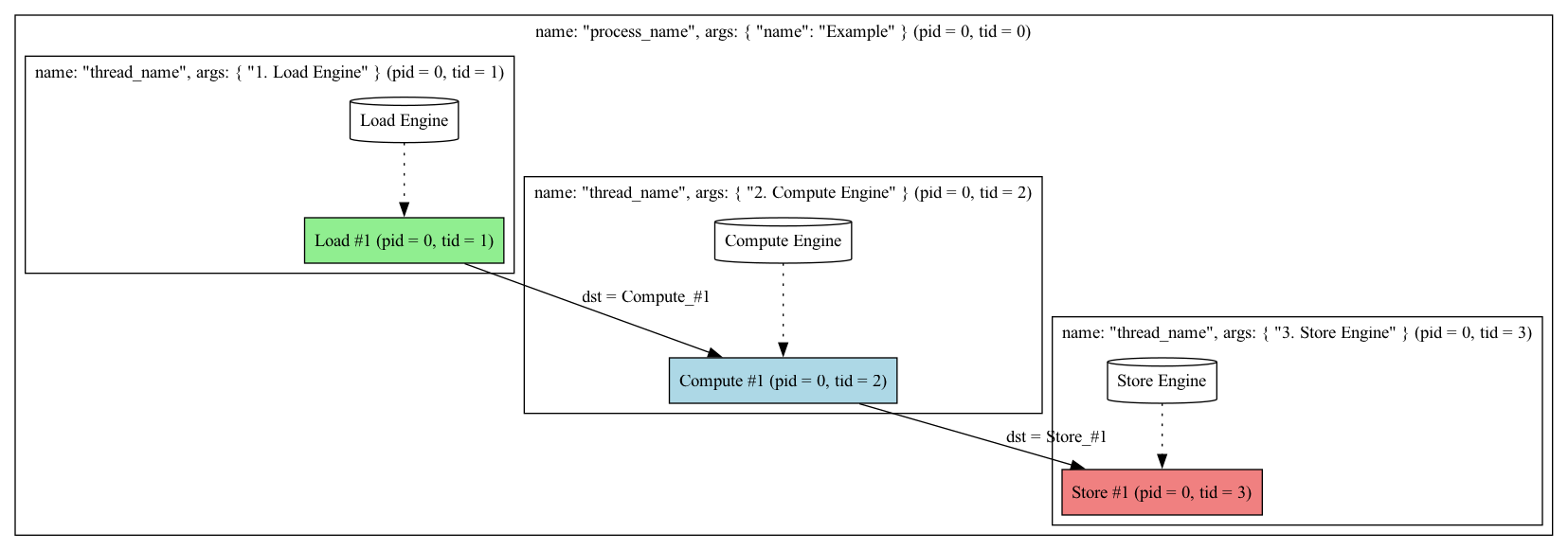
The trace events structure is organized from top level down as: process → thread → event. A process can be thought of as the current Example, while threads represent the vertical lanes within that process. In our example, we have threads for “1. Load Engine”, “2. Compute Engine”, “3. Store Engine”, and “4. Memory Bandwidth”.

Here’s a simple structural diagram for easier understanding:

Initializing Process and Threads

First, we need to initialize the processes and threads. Using ph: "M", which stands for “metadata”. When this phase is selected, the viewer interprets the event based on the “name” field to determine whether it’s a process or a thread. For a process, set name to "process_name". Similarly, for a thread, set it to "thread_name". And the actual display name is specified in the args.name field.

{ "name": "process_name", "ph": "M", "pid": 0, "tid": 0, "args": { "name": "Example" } },
{ "name": "thread_name", "ph": "M", "pid": 0, "tid": 1, "args": { "name": "1. Load Engine" } },
{ "name": "thread_name", "ph": "M", "pid": 0, "tid": 2, "args": { "name": "2. Compute Engine" } },
{ "name": "thread_name", "ph": "M", "pid": 0, "tid": 3, "args": { "name": "3. Store Engine" } },
{ "name": "thread_name", "ph": "M", "pid": 0, "tid": 4, "args": { "name": "4. Memory Bandwidth" } },

You must also set the pid and tid. While a process doesn’t require a tid. If you want a thread to belong to a specific process, the thread’s pid must match the process’s pid.

Duration Events

Next, we’ll introduce two types of events. For simple duration events, you can use two different approaches:

1. Begin/End Pairs (“B” and “E”)

This marks the beginning and end of an event separately. The viewer draws a rectangle using the ts values to show the event’s execution from start to finish. The tid must match the corresponding thread. For example, since we initialized the Load Engine at tid = 1, the event’s tid must also be set to 1. The same applies to pid. The cat (category) field helps you filter and find specific categories, though we just set to a meaningless name.

{ "name": "Load_#1", "cat": "foo", "ph": "B", "ts": 10000, "pid": 0, "tid": 1, "args": ...},
{ "name": "Load_#1", "cat": "foo", "ph": "E", "ts": 20000, "pid": 0, "tid": 1, "args": ...},

2. Complete Events (“X”)

Alternatively, you can use ph: "X" to represent an event with a single entry instead of a pair. This approach uses both ts and dur. For example, if ts is 100 and dur is 50, the event spans the time range [100, 150].

This is typically used when the execution time is known in advance at compile time. For instance, in ion-based quantum computing systems, pulse duration determines the rotation angle, requiring precise timing control. In such systems, all timing is known at compile time, so you know exactly how long each event will take. Similarly, in simulation systems with cost models, you can estimate the execution duration for a given computation. Using this phase can reduce JSON data size, which is quite beneficial.

{
  "name": "Load_#1",
  "cat": "foo",
  "ph": "X",
  "ts": 10000,
  "dur": 10000,
  "pid": 0,
  "tid": 1,
  "args": { "dest": "Compute_#1" }
}

Counter Events (“C”)

Counter events are used to represent continuous state changes, such as memory bandwidth in our chart. The value changes continuously but only updates at specific time points. Each event sets a value at a given timestamp. In the chart, we set the “GB/s” parameter to 40 at ts of 14000 (ns):

{ "name": "BW", "ph": "C", "ts": 14000, "pid": 0, "tid": 4, "args": { "GB/s": 40 } },

Nested Events

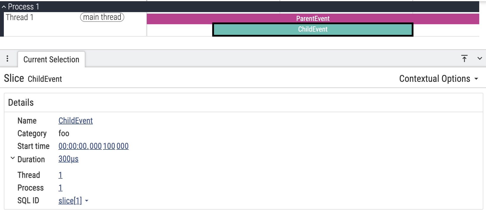
There’s another display method we haven’t shown in the chart yet: nested events.

{
  "traceEvents": [
    { "name": "ParentEvent", "cat": "foo", "ph": "X", "ts": 1000, "dur": 500, "pid": 1, "tid": 1 },
    { "name": "ChildEvent", "cat": "foo", "ph": "X", "ts": 1100, "dur": 300, "pid": 1, "tid": 1 }
  ]
}

The display effect is shown below. You can place two differently named events with overlapping times on the same tid, and both events will be displayed in the same area stacked vertically, rather than being separated.

Good! 🎉 Until now, we cover all the basic elements for expressing trace events. I think it’s far enough for most of the scenarios.

Pitfalls

There are some traps when using trace events that you should be aware of:

Time Unit Configuration: All time settings use microseconds (µs) as the unit. For the original chrome://tracing, you can force the display of event details to show nanoseconds (ns) by setting "displayTimeUnit": "ns". However, the timeline axis and other displays will use milliseconds (ms) 🤯, neither nanoseconds nor microseconds. Therefore, when generating this data, you must use microseconds as the data standard, but be aware that the display uses milliseconds. Even if you set "displayTimeUnit": "ns", it only changes the internal information shown when you click on an event, not the external display. This is definitely one of the most confusing design I’ve encountered.
Time Normalization: The first ts value will be normalized to 0. Therefore, even if you set the first event’s ts to 100, the display will still show it starting at 0. This is because the trace viewer was originally designed for use cases like web page operations and Android tracing, where timestamps often start at very high values. The leading empty space would be meaningless.